Project IV - MNIST Image Classification
In this project we are going to create a very simple neural network (linear classifier) to identify the handwritten digits from the MNIST database - often considered the “Hello World” problem in neural networks. In this problem we are given grayscale images of size 28 × 28 showing handwritten digits and are going to classify them into the 10 classes 0 - 9, depending on the digit depicted in the image. The MNIST database consists of 60.000 images to train your network on and 10.000 images to test the quality (accuracy) of the resulting network. For all images the correct label 0 - 9 is part of the database. There exist many of-the-shelf modules for this problem in Python, e.g. Keras, TensorFlow, scikit, and PyTorch, but in this project we are going to build a solution using pure Python from scratch.
A good introduction to the topic are the following four videos from the YouTube channel by 3BLUE1BROWN: Neural Network (19:13), Gradient Descend (21:00), Backpropagation (13:53), and Backpropagation Calculus (10:17). The few mathematical equations required in this project for performing simple backpropagation are stated explicitly below.
You are not allowed to use NumPy, Keras, etc. in the questions below (if not stated otherwise).
The first group of tasks concerns reading the raw data and visualizing them.
- From yann.lecun.com/exdb/mnist/ download the following four files:
- t10k-images.idx3-ubyte.gz (1.6 MB)
- t10k-labels.idx1-ubyte.gz (4.4 KB)
- train-images.idx3-ubyte.gz (9.6 MB)
- train-labels.idx1-ubyte.gz (28.3 KB)
-
Make a function
read_labels(filename)to read a file containing labels (integers 0-9) in the format described under FILE FORMATS FOR THE MNIST DATABASE. The function should return a list of integers. Test your method on the files t10k-labels.idx1-ubyte.gz and train-labels.idx1-ubyte.gz (the first five values of the 10.000 values in t10k-labels.idx1-ubyte.gz are [7, 2, 1, 0, 4]). The function should check if the magic number of the file is 2049.Hint: Open the files for reading in binary mode by providing
openwith the argument'rb'. You can either uncompress the files using a program like 7zip, or work directly with the compressed files using thegzipmodule in Python. In particulargzip.openwill be relevant. To convert 4 bytes to an integerint.from_bytesmight become useful. -
Make a function
read_images(filename)to read a file containing MNIST images in the format described under FILE FORMATS FOR THE MNIST DATABASE. Test your method on the files t10k-images.idx3-ubyte.gz and train-images.idx3-ubyte.gz. The function should return a three dimensional list of integers, such that images[image][row][column] is a pixel value (an integer in the range 0..255), and 0 ≤ row, column < 28 and 0 ≤ image < 10000 for t10k-images.idx3-ubyte.gz. The function should check if the magic number of the file is 2051. - Make a function
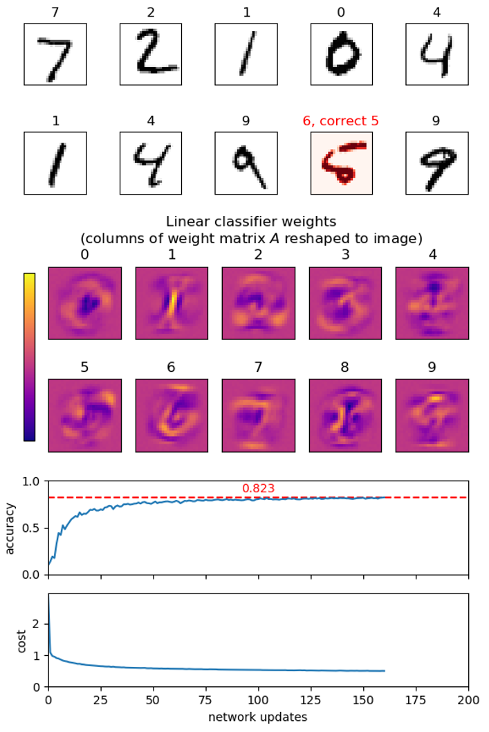
plot_images(images, labels)to show a set of images and their corresponding labels as titles usingimshowfrommatplotlib.pyplot. Show the first few images from t10k-images.idx3-ubyte.gz with their labels from t10k-labels.idx1-ubyte.gz as titles. Remember to select an appropriate colormap forimshow.
A linear classifier consists of a pair (A, b), where A is a weight matrix of size 784 × 10 and b is a bias vector of length 10. An image containing 28 × 28 pixels is viewed as a vector x of length 784 (= 28 · 28), where the pixel values are scaled to be floats in the range [0, 1]. In the following we denote this representation an image vector. The prediction by the classifier is computed as
a = xA + b,
where a = (a0, …, a9), i.e. the result of the vector-matrix product xA, that results in a vector of length 10, followed by a vector-vector addition with b. The predicted class is the index i, such that ai is the largest entry in a.
In the follow we will apply the cost measure mean squared error to evalutate how close the output a = xA + b of a network (A, b) is for an input x to the correct answer y, where we assume that y is the categorical vector of length 10 for the correct label, i.e. yi = 1 if i = label, and 0 otherwise:
cost(a, y) = sumi ((ai - yi)2) / 10
We use the mean squared error because is has an easy computable derivative, although better cost functions exist for this learning problem, e.g. softmax.
Below you will be asked to compute weights (A, b) using back propagation. To get started, a set of weights (A, b) is available as mnist_linear.weights. The weights were generated using the short program mnist_keras_linear.py using the neural networks API Keras running on top of Google’s TensorFlow. The network achieves around 92% accuracy on the MNIST test set (you should not expect to reach this level, since this network is trained using the softmax cost function).
- Optional: You should be able to reproduce a similar weight file (but not exactly the same) by runing the script, after pip installing tensorflow. This is not part of the project.
The second group of tasks is to load and save existing linear classifier networks and to evaluate their performance, together with various helper functions. In the following we assume the vector b to be represented by a standard Python list of floats and the matrix A to be represented by a list-of-lists of floats.
-
Write functions
linear_load(file_name)andlinear_save(file_name, network)to load and save a linear classifiernetwork= (A, b) using JSON. Test your functions on mnist_linear.weights. -
Write function
image_to_vector(image)that converts an image (list-of-lists) with integer pixel values in the range [0, 255] to an image vector (list) with pixel values being floats in the range [0, 1]. -
Write functions for basic linear algebra
add(U, V),sub(U, V),scalar_multiplication(scalar, V)multiply(V, M),transpose(M)whereVandUare vectors andMis a matrix. Include assertions to check if the dimensions of the arguments toaddandmultiplyfit. -
Write a function
mean_square_error(U, V)to compute the mean squared error between two vectors.Examples:
mean_square_error([1,2,3,4], [3,1,3,2])shoule return2.25. -
Write function a function
argmax(V)that returns an index into the listVwith maximal value (corresponding tonumpy.argmax).Example:
argmax([6, 2, 7, 10, 5])should return3. -
Implement a function
categorical(label, classes=10)that takes a label from [0, 9] and returns a vector of lengthclasses, with all entries being zero, except entrylabelthat equals one. For an image with this label, the categorical vector is the expected ideal output of a perfect network for the image.Example:
categorical(3)should return[0,0,0,1,0,0,0,0,0,0]. -
Write a function
predict(network, image)that returns xA + b, given a network (A, b) and an image vector. -
Create a function
evaluate(network, images, labels)that given a list of image vectors and corresponding labels, returns the tuple (predictions, cost, accuracy), where predictions is a list of the predicted labels for the images, cost is the average of mean square errors over all input-output pairs, and accuracy the fraction of inputs where the predicted labels are correct. Apply this to the loaded network and the 10.000 test images in t10k-images. The accuracy should be around 92%, whereas the cost should be 230 (the cost is very bad since the network was trained to optimze the cost measure softmax).Hint. Use your
argmaxfunction to convert network output into a label prediction. -
Extend
plot_imagesto take an optional argumentpredictionthat is a list of predicted labels for the images, and visualizes if the prediction is correct or wrong. Test it on a set of images from t10k-images and their correct labels from t10k-labels. -
Column i of matrix A contains the (positive or negative) weight of each input pixel for class i, i.e. the contribution of the pixels towards the image showing the digit i. Use
imshowto visualize each column (each column is a vector of length 784 that should be reshaped to an image of size 28 × 28).
The third group of tasks is to train your own linear classifier network, i.e. to compute a matrix A and a vector b.
-
Create function
create_batches(values, batch_size)that partitions a list of values into batches of size batch_size, except for the last batch, that can be smaller. The list should be permuted before being cut into batches.Example:
create_batches(list(range(7)), 3)should return[[3, 0, 1], [2, 5, 4], [6]]. -
Create a function
update(network, images, labels)that updates the networknetwork= (A, b) given a batch of n image vectors and corresponding output labels (performs one step of a stochastical gradient descend in the 784 · 10 + 10 = 7850 dimensional space where all entries of A and b are considered to be variables).For each input in the batch, we consider the tuple (x, a, y), where x is the image vector, a = xA + b the current network’s output on input x, and y the corresponding categorical vector for the label. The biases b and weights A are updated as follows:
bj
-=σ · (1 / n) · ∑(x,a,y) 2 · (aj - yj) / 10Aij
-=σ · (1 / n) · ∑(x,a,y) xi · 2 · (aj - yj) / 10For this problem an appropriate value for the step size σ of the gradient descend is σ = 0.1.
In the above equations 2 · (aj -yj) / 10 is the derivative of the cost function (mean squared error) wrt. to the output aj, whereas xi · 2 · (aj - yj) / 10 is the derivative of the cost function w.r.t. to Aij — both for a specific image (x, a, y).
-
Create a function
learn(images, labels, epochs, batch_size)to train an initially random network on a set of image vectors and labels. First initialize the network to contain random weights: each value of b to be a uniform random value in [0, 1], and each value in A to be a uniform random value in [0, 1 / 784]. Then performepochsepochs, each epoch consiting of partitioning the input into batches ofbatch_sizeimages, and callingupdatewith each of the batches. Try running your learning function withepochs=5andbatch_size=100on the MNIST training set train-images and train-labels.Hint. The above computation can take a long time, so print regularly a status of the current progress of the network learning, e.g. by evaluating the network on (a subset of) the test images t10k-images. Regularly save the best network seen so far.
Here are some additional optional tasks. Feel free to come up with your own (other networks, other optimization strategies, other loss functions, …).
-
Optional. Instead of using the mean squared error as the cost function try to use the categorical cross entropy (see e.g. this blog): On output a where the expected output is the categorical vector y, the categorical cross entropy is defined as CE(y, softmax(a)), where softmax(a)i = eai / (∑j eaj) and the cross entropy is defined as CE(y, â) = - ∑i (yi · log âi).
In
updatethe derivative of the cost function w.r.t. output aj should be replaced by eaj /(∑k eak) - yj.Note. softmax(a) is a vector with the same length as a with values having the same relative order as in a, but elements are scalled so that softmax(a)i ∈ ]0,1[ and 1 = ∑i softmax(a)i. Furthermore, since y is categorical with yi = 1 for exactly one i, CE(y, softmax(a)) = log(∑j eaj) - ai.
-
Optional. Visualize the changing weights, cost, and accuracy during the learning.
Hint. You can use
matplotlib.animation.FuncAnimation, and let the provided function apply one batch of training data to the network for each call. -
Optional: Redo the above exercises in Numpy. Create a generic method for reading IDX files into NumPy arrays based on the specification THE IDX FILE FORMAT. Data can be read from a file directly into a NumPy array using
numpy.fromfileand an appropriate dtype.Hint.
np.argmax(test_images.reshape(10000, 28 * 28) @ A + b, axis=1)computes the predictions for all tests images, if they are all in one NumPy array with shape (10000, 28, 28). -
Optional: Compare your pure Python solution with your Numpy implementation (if you did the above optional task) and/or the solution using Keras, e.g. on running time, accuracy achieved, epochs.
-
Optional: Try to take a picture of your own handwritten letters and see if your program can classify your digits. It is important that you preprocess your images to the same nomalized format as the original MNIST data: Images should be 28 × 28 pixels where each pixel is represented by an 8-bit greyscale value where 255 is black and 0 is white. The center of mass should be in the center of the image. In the test data all images were first scaled to fit in a 20 × 20 box, and then padded with eight rows and columns with zeros to make the center of mass the center of the image, see yann.lecun.com/exdb/mnist.
Hint:
PIL.Image.resizefrom thePillow(Python Imaging Library) might be usefull. Remember to set the resampling filter to BILINEAR.