Project III - Simulations of NMR spectra of proteins
A fingerprint of a protein can be obtained by a nuclear magnetic resonance (NMR) experiment with a given spectrometer frequency (inputMHz). The fingerprint will be a spectrum of intensities over the frequency range.
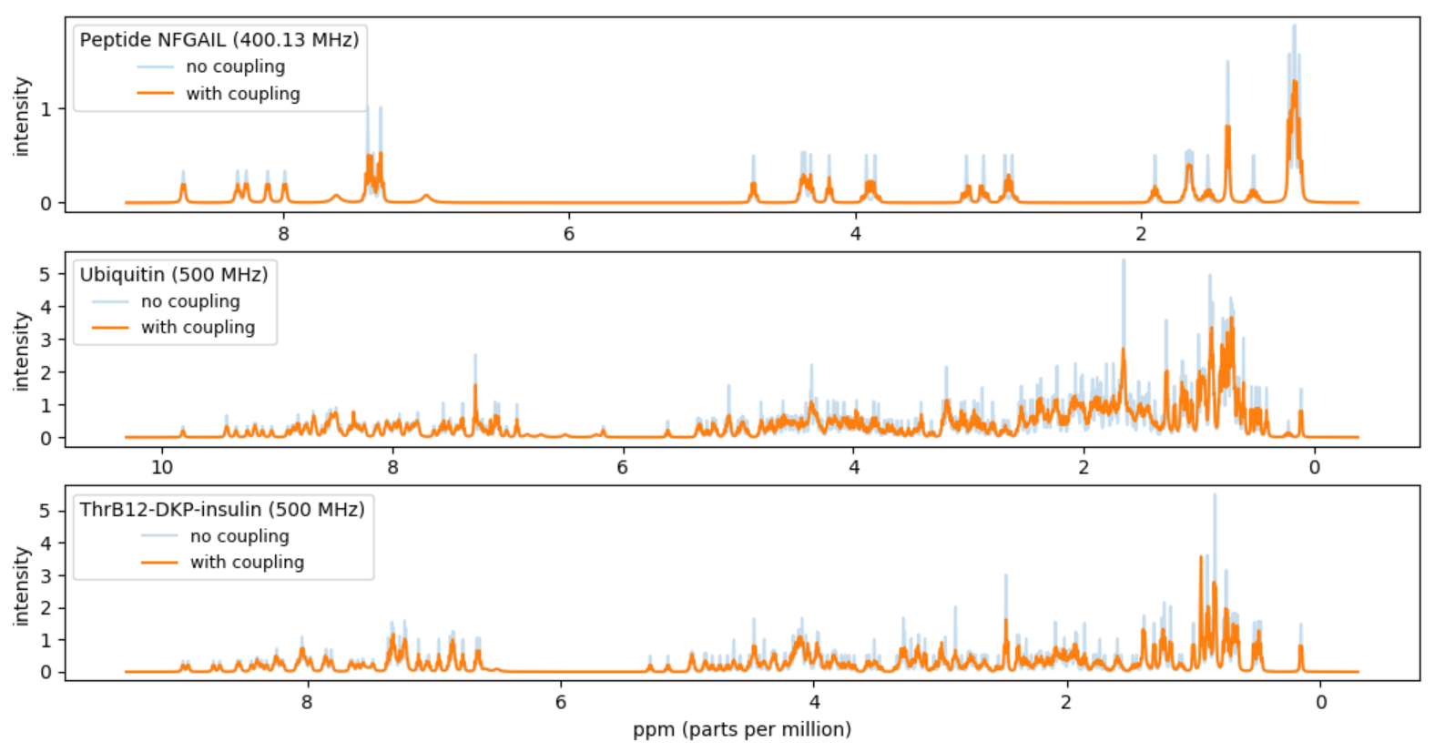
In this project you should compute a simulated approximation of the NMR fingerprint of a protein. In particular you should try to reproduce Figure 5(b) in [1].
The approximate fingerprint of a protein should be computed based on data available for the chemical shifts of the H-atoms in the protein and coupling data for H-atoms inside amino acids. We will approximate the spectrum with the sum of a set of Lorentz lines.
Protein molecules consist of one or more chains of amino acid residues. In the mandatory part of this project we will only consider proteins with one chain. Each amino acid in such a chain is identified by a a unique Seq_ID, an integer starting with one for the first amino acid in the sequence. The amino type is identified by Comp_ID (three letter abbreviation). Each atom in an amino acid has again a unique Atom_ID, where the first character is the atom type (i.e. in this project always H).
This project consists of the below tasks. Please remember to split your code into logical units, e.g. by introducing functions for various (recurring) subtasks.
-
Download the files NFGAIL.csv, couplings.csv and 68_ubiquitin.csv.
-
The simplest Lorentz line is the function
L(x) = 1 / (1 + x2) .
Make a function
Lorentzthat given x returns L(x), where x can be either an integer, a float or a Numpy array. In the case of a Numpy array the function should be computed pointwise for each value. Plot the function for x ∈ [−10, 10] usingmatplotlib.pyplotHint: use
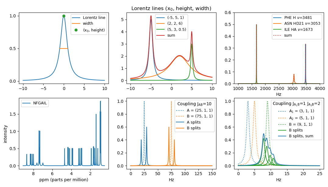
numpy.linspace.The function L has a maximum in (0, 1). We let (x0, height) denote the coordinates of the maximum of a Lorentz line. We let the width of a Lorentz line be the width of the peak at height height / 2, sometimes denoted full width half height (FWHH). The function L has width 2. Note that the area below L is π = ∫(−∞,+∞) L(x) dx.
-
Generalize your function
Lorentzto take (optional keyword) arguments for x0, height and width. The resulting function should computeLx0, height, width(x) = height / (1 + (2 · (x − x0) / width)2) .
Plot three Lorentz lines for the parameters (x0, height, width) being (-5, 5, 1), (2, 2, 6), and (5, 3, 0.5) for x ∈ [-10,10]. Plot also the sum of the three curves. Note that the area below a general Lorentz line is π · height · width / 2.
-
Our basic assumption is that each atom in a molecule contributes approximately one Lorentz line to the spectra. We will not use the same Lorentz parameters for all atoms. The width will e.g. depend on the atom_id and possibly also on the amino acid the atom is part of.
Make a function
peak_width(amino, atom_id)that returns the width for an atom in a specic amino acide and having a specific atom_id. If atom_id is H the width is 6 (note this is only when the atom_id is H and not for all atoms of type H). If (amino, atom_id) is one of the following four pairs (ASN, HD21), (ASN, HD22), (GLN, HE21), (GLN, HE22) the width is 25. For all other atom_id’s the width is 4. -
We will denote a Lorentz line a peak and identify it by the triple (x0, height, width).
For an atom (amino, atom_id) with assigned chemical shift value x0 (in Hz) we create a peak with width determined by
peak_widthand maximum value at (x0, height), where height is chosen such that the area below the Lorentz line is π.Create a function
atom_peak(amino, atom_id, Hz)that returns the triple for the corresponding peak, where x0 =Hz= the chemical shift in Hz.Plot the peaks for the three atoms and assigned chemical shifts (PHE, H, 3481 Hz), (ASN, HD21, 3053 Hz), and (ILE, HA, 1673 Hz). Furthermore plot the sum of the three peaks.
-
Create a function
read_moleculethat reads a list of atoms for a single protein from a CSV-file, where each row stores the description of an atom in the protein (most of the columns will not be used in this project). You can e.g. store each atom as a dictionary mapping column names to row values (Hint: usezip) or read the file as apandasdata frame. -
Read in the molecule description of the NFGAIL protein from the file NFGAIL.csv. For each of the 44 H-atoms create a peak assuming inputMHz = 400.13 MHz. The relevant columns are
Atom_ID,Comp_ID(= amino acid), andVal. The columnValis the chemical shift in ppm, parts per million, but this value should be converted to Hz for calculations. To get the shift in Hz, multiply theValvalue by inputMHz.Plot the sum of the peaks. Make the unit of the x-axis ppm (= Hz / inputMHz) and make the x-axis be decreasing from left to right.
Note. In the protein descriptions there is no H-atom listed for the first amino acid, since this H-atom will not be visible in the NMR spectra as it is in fast exchange with water.
-
To get a more refined spectrum we will take couplings between atoms into account. Between two H-atoms A and B in an amino acid (i.e. two peaks) there can be a coupling with magnitude JAB, in the following just denoted J, that influences the resulting spectrum. (Many other factors influence the spectrum, but we will happily ignore these in our simulations). The coupling between A and B causes both peaks to be split into two new peaks Ainner, Aouter, Binner and Bouter, where Binner is closer to A than B, and Bouter is further away from A than B. In the following we only consider Binner and Bouter (A is handled symmetrically).
The height of Bouter is smaller than the height of Binner, the sum of their heights equals the height of B, and their width equals the width of B. Assume A and B have their maximum at_x_0 = νA and x0 = νB, respectively. Let
Q = sqrt((νA − νB)2 + J2)
νm = (νA + νB) / 2
σ = 1 if νA < νB, −1 otherwise
αinner = (1 + J / Q) / 2
αouter = (1 − J / Q) / 2 .
The points Binner and Bouter are given by
νBinner = νm + σ · (Q − J) / 2 , heightBinner = heightB · αinner , widthBinner = widthB ,
νBouter = νm + σ · (Q + J) / 2 , heightBouter = heightB · αouter , widthBouter = widthB .
Make a function
apply_coupling(A, B, J)that takes two peaksAandBand computes the effect ofAonB, when the coupling has magnitudeJ. Returns the list of the two peaksBinner andBouter thatBis split into. IfJ= 0 or x0(A) = x0(B), then only[B]is returned.Plot the four peaks resulting from the mutual coupling of two peaks A = (25, 1, 1) and B = (75, 1, 1) with J = 10.
-
If an atom has couplings with several atoms the computations become slightly more involved. Assume B has couplings with k atoms A1, A2, …, Ak with magnitudes J1, J2, …, Jk, respectively. In general the peak for B will be split into 2k peaks.
The basic idea is to start with the peak B. Applying the coupling of B and A1 with magnitude J1 on B results in a list L1 with at most two peaks. Applying the coupling of B and A2 with magnitude J2 on each B’ ∈ L1 results in the list L2 with at most four peaks. Applying A3 on the peaks in L2 results in eight peaks L3, etc.
Applying the coupling between Ai and B with magnitude J on a peak B’ ∈ Li − 1 is done as applying A on B, except that the final computation of the points B’inner and B’outer are given by
νB’inner = νB’ − νB + νm + σ · (Q − J) / 2 , heightB’inner = heightB’ · αinner , widthB’inner = widthB
νB’outer = νB’ − νB + νm + σ · (Q + J) / 2 , heightB’outer = heightB’ · αouter , widthB’outer = widthB
Extend your function
apply_couplingto also be able to take a peak B’ as an additional (optional) fourth argument. Note that for B’ = B the function should return the same value as without the B’ argument.Make a function
apply_couplings([(A1, J1), (A2, J2), ..., (Ak, Jk)], B)to apply all couplings onB.Plot the four peaks and their sum resulting from applying A1 = (3, 1, 1) and A2 = (5, 1, 1) on B1 = (9, 1, 1) with magnitude J1 = 1 and J2 = 2, respectively. Note that permuting the list of (Ai, Ji)s should result in the same set of peaks for B.
-
Make a function to read the file couplings.csv that for each of the 20 amino acids contains the coupling magnitudes among the H-atoms inside the amino acid.
-
Make a function
split_compsthat splits a list of atoms for a protein into a list of sublists, one sublist for each amino acid on the chain, i.e. split the list into sublists based on Seq_ID. -
Make a function
comp_peaks(comp, couplings, input_MHz)that computes the peaks for all atoms in a amino acid (comp) by taking the table of couplings from couplings.csv into acount. -
Make a function
protein_peaks(atoms, couplings, input_MHz)that takes a list of atoms for a protein, a table of couplings, and a frequency inputMHz and returns the resulting peaks by applying all couplings.Apply the function to the data from NFGAIL.csv with inputMHz = 400.13 MHz.
Plot the sum of the resulting 542 peaks. Make the unit of the x-axis ppm (= Hz / inputMHz) and make the x-axis be decreasing from left to right.
Your result should be a reproduction of 5(b) in [1].
The following tasks are optional.
In the previous tasks you were given CSV-files with the description of proteins only containing one chain. The following tasks ask you to download protein descriptions from the Biological Magnetic Resonance Data Bank (BMRB, bmrb.wisc.edu containing an arbitrary number of chains. In the data bank each data set for a molecule has a unique Entry_ID value. Each chain is identified by a unique Entity_ID. Each amino acid in a chain has a unique Seq_ID (and amino type Comp_ID) and each atom in an amino acid has again a unique Atom_ID.
-
Download the file Atom_chem_shift.csv (700+ MB) from www.bmrb.wisc.edu > Bulk access > CSV relational data tables. This file contains the atom shift data for all data sets on the web site.
-
Write a function
csv_extractthat given a value Entry_ID, from Atom_chem_shift.csv extracts all rows with value Entry_ID in columnEntry_IDand outputs the resulting rows to a new CSV-file. Test this with Entry_ID = 68 and Entry_ID = 6203. The result for Entry_ID = 68 should be the 556 atoms as provided in the file [68ubiquitin.csv](68_ubiquitin.csv) (but with additional columns). The result for _Entry_ID = 6203 should be a file with a header row plus 329 data rows (atoms) for ThrB12-DKP-insulin.Hint: Avoid reading the whole table into memory. If you e.g. read the complete table using Pandas, the data will take up memory ≈ 3 × file size. Instead scan through the file using the
csvmodule and only have the current line in memory. Scanning through the 700+ MB should be possible within in the order of a minute. -
Update the function
split_compsto be able to handle more than one chain of amino acids. In particular each comp should now be identified not only by Seq_ID but by the pair (Entity_ID, Seq_id). -
Extract data for ThrB12-DKP-insulin (
Entry_ID= 6203) from Atom_chem_shift.csv and plot the resulting simulated spectrum for inputMHz = 500 MHz. Note that the data for ThrB12-DKP-insulin consists of two chains of 131 and 198 atoms, respectively. You can find the Entry_ID value for your favorite protein by searching the BMRB data base at www.bmrb.wisc.edu.
| Protein | Uncoupled peaks | Coupled peaks |
|---|---|---|
| NFGAIL | 44 | 542 |
| Ubiquitin | 556 | 6805 |
| ThrB12-DKP-insulin | 329 | 3338 |
References
[1] Fast simulations of multidimensional NMR spectra of proteins and peptides. Thomas Vosegaard. Magnetic Resonance in Chemistry. 56(6), 438-448, 2018. DOI: 10.1002/mrc.4663.