Introduction to Programming and Scientific Applications (Spring 2019)
Final project
The goal of the final project is to do some concrete Python implementation and documenting it in a short report. The project can be done in groups with 1-3 students. There are three deliverables for the final project that should be handed in:
- Python code. Either plain Python 3 code in one or more .py files, or Python 3 code embedded into a Jupyter file.
- A report - maximum 4 pages. The front page must contain the information listed below (the front page does not count towards the page count).
- Visualization of data. E.g. matplotlib output. The plots should be included in an appendix to the report, that does not count towards the page count, or alternatively embedded in a Jupyter file.
Evaluation of handin
The project deliverables will be scored according to the following rubric:
| Deliverable | Not present 0% |
Many major shortcomings 25% |
Some major weaknesses 50% |
Minor weaknesses 75% |
Solid 100% |
|---|---|---|---|---|---|
| Code 50% |
No code, or code where no part computes the required | Some elementary parts of the code work, but significant parts do not work | Most essential parts of the code work, but the code does not completely solve the problem addressed | Overall good code, but space for improvement, e.g. missing documentation, code could be made clearer | Complete code, well structured, good use of modules, clear variable names, good documentation, PEP8 compliant |
| Visualization 25% |
No visualization | Very few or very unclear visualizations | Some visualizations illustrating basic idea | Overall good visualization but some details could have been more clear | Clear visualizations documenting the problem being solved and supporting the conclusions drawn |
| Report 25% |
No report | Very unpolished report, missing structure, no clear conclusions, major misunderstandings | The basic ideas are described but details are missing | Overall good report but for some aspects the level of detail/precision could be higher | Solid report, containing reflection upon the implementation done, discussion of the Python modules used, the design choices made, discussion of the structure of the code, what were the hardest parts, what is missing, and discussion of testing and visualization |
Project report
The project report must contain the below front page (not counted in the 4 pages). Make sure you read and understand the note on plagiarism. The report can be written in Danish and English.
Project descriptions
You can choose any of the below projects as your final project.
Project I - Geometric medians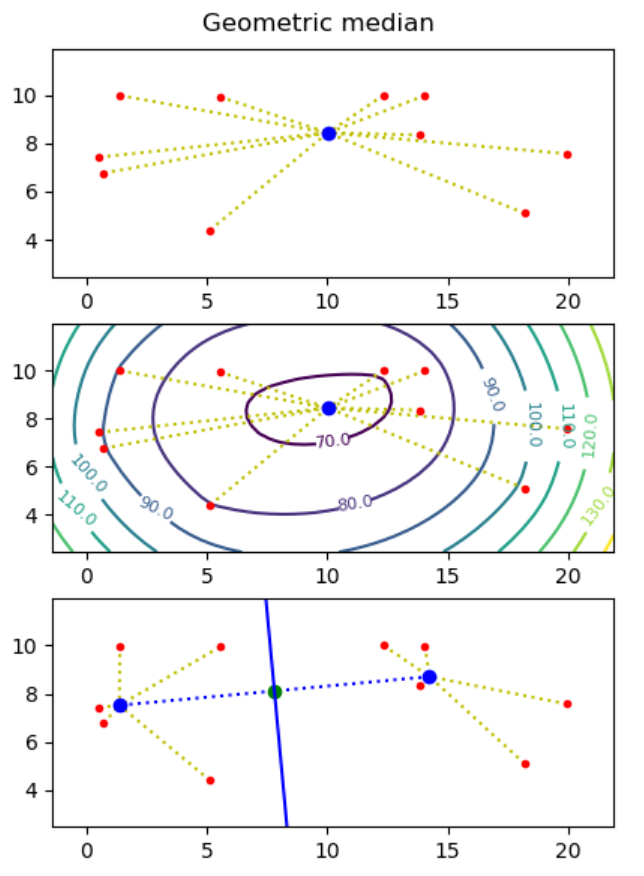
Motivation: Assume you want to build a drone tower from where to deliver parcels to costumers, and you know the destinations (points) where to deliver parcels. What is the optimal placement of the tower, if each drone can at most carry one parcel and needs to return to the tower between each delivery?
The geometric median of a point set S = { p1, ..., pn } in the plane is a point q (not necessarily a point in S), that minimizes the sum of distances to the points, i.e. minimizes ∑i=1..n |pi - q|, where |p - q| = ((px - qx)2 + (py - qy)2)0.5.
-
Create a function geometric_median that given a list
of points computes the geometric median of the point set.
Hint. Use the minimize function from the module scipy.optimize. - Make representative visualizations that show both the input point sets and the computed geometric medians. Examples should include point sets with two and three points, and a random point set.
- Use the matplotlib plotting function contour to plot a contour map to illustrate that it is the correct minimum that mas been found (the z-value for a point (x, y) in the contour map is the sum of the distances from (x, y) to all input points).
Next we want to find two points q1 and q2 such that the perpendicular bisector of q1 and q2 partitions the point set into the points closest to q1 and those closest to q2. We want to find two points q1 and q2 such that the sum of distances to the nearest point of q1 and q2 is minimized, i.e. ∑i=1..n min(|pi - q1|, |pi - q2|) is minimized.
To solve this problem one essentially has to consider all possible bisection lines, and to find the geometric median on both sides of the bisector, e.g. using the algorithm from question a). Assuming no three points are on a line, it is sufficient to consider all n(n-1)/2 bisector lines that go through two input points, and for each bisector line to consider the two cases where the two points on the line both are considered to be to the left or to the right of the line.
- Create a function two_geometric_medians that give a list of points p1, ..., pn computes two points q1 and q2 minimizing ∑i=1..n min(|pi - q1|, |pi - q2|). It can be assumed that no three points are on a line.
- Visualize your solution, showing imput points, q1 and q2, and the perpendicular bisector between q1 and q2.
- [optional] Extend your solution to handle the case where three or more points can be on a line. E.g. what is your solution if you have four points on a line?
Project II - Portfolio optimization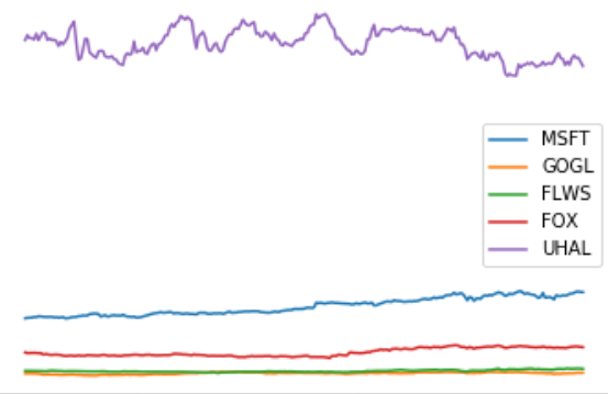
We consider the problem of choosing a long term stock portfolio, given a set of stocks and their price over some period under risk aversion parameter γ > 0.
Assume there are m stocks to be considered. The portfolio will be represented by a vector w ∈ ℝm, such that ∑i=1..m wi = 1. If wi > 0, you use a fraction wi of your total money to buy the i'th stock, while wi < 0 represent shorting that stock. In both cases we assume the stock is bought/shorted for the entire period.
Let pj,i represent the price of the i'th stock at time step j. If there are n time steps, then p ∈ ℝn×m is a matrix.
Let rj,i represent the fractional reward of stock i at time step j, i.e. rj,i = (pj,i - pj-1,i) / pj-1,i for j > 1.
We make the (unrealistic) assumption that we can model r by a random variable, distributed as a multivariate Gaussian with estimated means,
μ = E[r] ≃ 1/n · ∑j=1..n rj
and estimated variances,
Σ = E[(r - μ)(r - μ)T] ≃ 1/n · ∑j=1..n [(rj - μ)(rj - μ)T]
The distribution of returns using some w is then
Rw = N(μw, σw2)
μw = wTμ
σw2 = wTΣw
Now, we want to maximize for a balance between high return μw and low risk σw2. This leads to the following optimization problem, where we ant to find the value w* of w maximizing the following expresion:
maximize wTμ - γwTΣw
subject to ∑i=1..m wi = 1
where γ controls the balance between risk and return. A high value of γ indicate we are willing to take low risk and vise versa.
In this project you should find w* for different values of γ and using real stock values of your choice. The project consists of the following three questions.
- We need a module for collecting stock values. For this you can e.g. use the module googlefinance or pandas-datareader (Warning: people have experienced problems with getting data using to the googlefinance API; if you are using another data source than googlefinance, then adjust the arguments to get_prices to your data source). Using this you should write a function get_prices([stock1, ..., stockk], step_size, period, exchange), that returns a tuple (stocks, p), where p[j, i] represents the opening price of stock i at time step j and stocks[i] is the name of the i'th stock. Make a plot of p, where each stock is labeled with its name, e.g. MSFT or GOGL. You should use at least five stocks.
-
Calculate r, μ and Σ using the formulas above and
the p calculated in question (a). Plot
the probability density function (pdf) of the return of each
stock.
Hint. The method normpdf from the module matplotlib.mlab might become convenient. -
Solve the optimization problem defined above for different values
of gamma, e.g. gammas = (np.arange(10) / 5) + 1, and plot
the pdf of each solution to a single plot with appropriate
legends. Finally create a scatter plot of how w* changes as
γ changes: For each value of γ plot the fraction of
each stock in the portfolio.
Project III - Simulations of NMR spectra of proteins
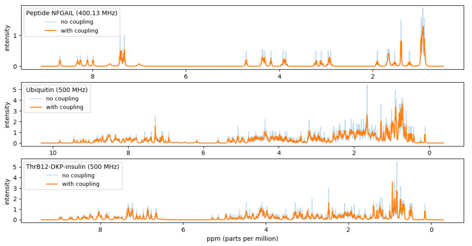
A fingerprint of a protein can be obtained by a nuclear magnetic resonance (NMR) experiment with a given spectrometer frequency (inputMHz). The fingerprint will be a spectrum of intensities over the frequency range. In this project you should compute a simulated approximation of the NMR fingerprint of a protein. In particular you should try to reproduce Figure 5(b) in [1]. The approximate fingerprint of a protein should be computed based on data available for the chemical shifts of the H-atoms in the protein and coupling data for H-atoms inside amino acids. We will approximate the spectrum with the sum of a set of Lorentz lines.
Protein molecules consist of one or more chains of amino acid residues. In the mandatory part of this project we will only consider proteins with one chain. Each amino acid in such a chain is identified by a a unique Seq_ID, an integer starting with one for the first amino acid in the sequence. The amino type is identified by Comp_ID (three letter abbreviation). Each atom in an amino acid has again a unique Atom_ID, where the first character is the atom type (i.e. in this project always H).
This project consists of the below tasks. Please remember to split your code into logical units, e.g. by introducing functions for various (recurring) subtasks.

- Download the files NFGAIL.csv, couplings.csv and 68_ubiquitin.csv.
-
The simplest Lorentz line is the function
L(x) = 1 / (1 + x2) . Make a function Lorentz that given x returns L(x), where x can be either an integer, a float or a Numpy array. In the case of a Numpy array the function should be computed pointwise for each value. Plot the function for x ∈ [−10, 10] using matplotlib.pyplot (Hint: use numpy.linspace). The function L has a maximum in (0, 1). We let (x0, height) denote the coordinates of the maximum of a Lorentz line. We let the width of a Lorentz line be the width of the peak at height height / 2, sometimes denoted full width half height (FWHH). The function L has width 2. Note that the area below L is π = ∫(−∞,+∞) L(x) dx. -
Generalize your function Lorentz to take (optional keyword) arguments for
x0, height and width.
The resulting function should compute
Lx0, height, width(x) = height / (1 + (2 · (x − x0) / width)2) . Plot three Lorentz lines for the parameters (x0, height, width) being (-5, 5, 1), (2, 2, 6), and (5, 3, 0.5) for x ∈ [-10,10]. Plot also the sum of the three curves. Note that the area below a general Lorentz line is π · height · width / 2. - Our basic assumption is that each atom in a molecule contributes approximately one Lorentz line to the spectra. We will not use the same Lorentz parameters for all atoms. The width will e.g. depend on the atom_id and possibly also on the amino acid the atom is part of. Make a function peak_width(amino, atom_id) that returns the width for an atom in a specic amino acide and having a specific atom_id. If atom_id is H the width is 6. If (amino, atom_id) is one of the following four pairs (ASN, HD21), (ASN, HD22), (GLN, HE21), (GLN, HE22) the width is 25. For all other atom_id's the width is 4.
- We will denote a Lorentz line a peak and identify it by the triple (x0, height, width). For an atom (amino, atom_id) with assigned chemical shift value x0 (in MHz) we create a peak with width determined by peak_width and maximum value at (x0, height), where height is chosen such that the area below the Lorentz line is π. Create a function atom_peak(amino, atom_id, MHz) that returns the triple for the corresponding peak, where x0 = MHz = the chemical shift in MHz. Plot the peaks for the three atoms and assigned chemical shifts (PHE, H, 3481 MHz), (ASN, HD21, 3053 MHz), and (ILE, HA, 1673 MHz). Furthermore plot the sum of the three peaks.
- Create a function read_molecule that reads a list of atoms for a protein from a CSV-file, where each row stores the description of an atom in a protein (most of the columns will not be used in this project). You can e.g. store each atom as a dictionary mapping column names to row values (Hint: use zip) or read the file as a pandas data frame.
- Read in the molecule description of the NFGAIL protein from the file NFGAIL.csv. For each of the 44 H-atoms create a peak assuming inputMHz = 400.13 MHz. The relevant columns are Atom_ID, Comp_ID (= amino acid), and Val. The column Val is the chemical shift in ppm, parts per million, but this value should be converted to MHz for calculations. To get the shift in MHz, multiply the Val value by inputMHz. Plot the sum of the peaks. Make the unit of the x-axis ppm (= MHz / inputMHz) and make the x-axis be decreasing from left to right.
-
To get a more refined spectrum we will take couplings between atoms into account.
Between two H-atoms A and B in an amino acid
(i.e. two peaks) there can be a coupling with
magnitude JAB, in the following just
denoted J, that influences the resulting spectrum. (Many
other factors influence the spectrum, but we will happily
ignore these in our simulations). The coupling between A
and B causes both peaks to be split into two new peaks
Ainner,
Aouter,
Binner and
Bouter,
where
Binner is closer to A than B,
and Bouter is further away from A than B.
In the following we only consider Binner
and Bouter (A is handled symmetrically).
The height of Bouter is smaller than the height of Binner,
the sum of their heights equals the height of B,
and their width equals the width of B.
Assume A and B have their maximum at
x0 = νA
and x0 = νB, respectively.
Let
Q = sqrt((νA − νB)2 + J2) The points Binner and Bouter are given by
νm = (νA + νB) / 2
σ = 1 if νA < νB, −1 otherwise
αinner = (1 + J / Q) / 2
αouter = (1 − J / Q) / 2 .νBinner = νm + σ · (Q − J) / 2 , heightBinner = heightB · αinner , widthBinner = widthB , Make a function apply_coupling(A, B, J) that takes two peaks A and B and computes the effect of A on B, when the coupling has magnitude J. Returns the list of the two peaks Binner and Bouter that B is split into. If J = 0 or x0(A) = x0(B), then only [B] is returned. Plot the four peaks resulting from the mutual coupling of two peaks A = (25, 1, 1) and B = (75, 1, 1) with J = 10.
νBouter = νm + σ · (Q + J) / 2 , heightBouter = heightB · αouter , widthBouter = widthB .
-
If an atom has couplings with several atoms the computations become slightly more involved. Assume B has couplings with k
atoms A1, A2, ..., Ak
with magnitudes
J1, J2, ..., Jk, respectively. In general the peak for B will be split into
2k peaks.
The basic idea is to start with the peak B.
Applying the coupling of B and A1 with magnitude J1 on B
results in a list L1 with at most two peaks.
Applying the coupling of B and A2 with magnitude J2 on each B' ∈ L1
results in the list L2 with at most four peaks. Applying A3 on the peaks in L2
results in eight peaks L3, etc.
Applying the coupling between Ai and B with magnitude J on a peak B' ∈ Li − 1 is done as applying A on B, except that the final computation of the points B'inner and B'outer are given byνB'inner = νB' − νB + νm + σ · (Q − J) / 2 , heightB'inner = heightB' · αinner , widthB'inner = widthB Extend your function apply_coupling to also be able to take a peak B' as an additional (optional) fourth argument. Note that for B' = B the function should return the same value as without the B' argument. Make a function apply_couplings([(A1, J1), (A2, J2), ..., (Ak, Jk)], B) to apply all couplings on B. Plot the four peaks and their sum resulting from applying A1 = (3, 1, 1) and A2 = (5, 1, 1) on B1 = (9, 1, 1) with magnitude J1 = 1 and J2 = 2, respectively. Note that permuting the list of (Ai, Ji)s should result in the same set of peaks for B.
νB'outer = νB' − νB + νm + σ · (Q + J) / 2 , heightB'outer = heightB' · αouter , widthB'outer = widthB
- Make a function to read the file couplings.csv that for each of the 20 amino acids contains the coupling magnitudes among the H-atoms inside the amino acid.
- Make a function split_comps that splits a list of atoms for a protein into a list of sublists, one sublist for each amino acid on the chain, i.e. split the list into sublists based on Seq_ID.
- Make a function comp_peaks(comp, couplings, input_MHz) that computes the peaks for all atoms in a amino acid (comp) by taking the table of couplings (from couplings.csv) into acount.
- Make a function protein_peaks(atoms, couplings, input_MHz) that takes a list of atoms for a protein, a table of couplings, and a frequency inputMHz and returns the resulting peaks by applying all couplings. Apply the function to the data from NFGAIL.csv with inputMHz = 400.13 MHz. Plot the sum of the peaks. Make the unit of the x-axis ppm (= MHz / inputMHz) and make the x-axis be decreasing from left to right. Your result should be a reproduction of 5(b) in [1].
The following tasks are optional.
In the previous tasks you were given CSV-files with the description of proteins only containing one chain. The following tasks ask you to download protein descriptions from the Biological Magnetic Resonance Data Bank (BMRB, bmrb.wisc.edu) containing an arbitrary number of chains. In the data bank each data set for a molecule has a unique Entry_ID value. Each chain is identified by a unique Entity_ID. Each amino acid in a chain has a unique Seq_ID (and amino type Comp_ID) and each atom in an amino acid has again a unique Atom_ID.
- Download the file Atom_chem_shift.csv (700+ MB) from www.bmrb.wisc.edu > Bulk access > CSV relational data tables. This file contains the atom shift data for all data sets on the web site.
- Write a function csv_extract that given a value Entry_ID, from Atom_chem_shift.csv extracts all rows with value Entry_ID in column Entry_ID and outputs the resulting rows to a new CSV-file. Test this with Entry_ID = 68 and Entry_ID = 6203. The result for Entry_ID = 68 should be the 556 atoms as provided in the file 68_ubiquitin.csv (but with additional columns). The result for Entry_ID = 6203 should be a file with a header row plus 329 data rows (atoms) for ThrB12-DKP-insulin. (Hint: Avoid reading the whole table into memory. If you e.g. read the complete table using Pandas, the data will take up memory ≈ 3 × file size. Instead scan through the file using the csv module and only have the current line in memory. Scanning through the 700+ MB should be possible within in the order of a minute.)
- Update the function split_comps to be able to handle more than one chain of amino acids. In particular each comp should now be identified not only by Seq_ID but by the pair (Entity_ID, Seq_id).
- Extract data for ThrB12-DKP-insulin (Entry_ID = 6203) from Atom_chem_shift.csv and plot the resulting simulated spectrum for inputMHz = 500 MHz. Note that the data for ThrB12-DKP-insulin consists of two chains of 131 and 198 atoms, respectively. You can find the Entry_ID value for your favorite protein by searching the BMRB data base at www.bmrb.wisc.edu.
References
[1] Fast simulations of multidimensional NMR spectra of proteins and peptides. Thomas Vosegaard. Magnetic Resonance in Chemistry. 56(6), 438-448, 2018. DOI: 10.1002/mrc.4663.
Project IV - Open topic
You can also define your own project. There are some aspects that needs to be addressed.
- Some minimal amount of Python 3 code must be produced.
- Use at least two different Python modules.
- Some data must be visualized, e.g using matplotlib, but any visualization module or domain specific library, like for chemistry, can be used.